Lab 2

Test Platform

• Model Name: MacBook Pro
• Chip: Apple M1 Pro
• Total Number of Cores: 8 (6 performance and 2 efficiency)
• Memory: 16 GB

Problem 1

The Local Output Variables Method

• This method of parallelizing matrix multiplication is analogous to the block-based method. It partitions the output matrix into blocks based on the number of threads the user wants and then assigns each block to a thread for independent computation.

• $p \times p$ threads, each thread $(i,j)$ “owning” the computation of a $C(i,j)$ block, is responsible for calculating its matrix product of corresponding tile from $A$ and $B$ and write the results to $C(i,j)$.

Results

• thread = 1 (Using lab 1's result):

  Number of FLOPs = 137438953472, Execution time = 835.089545 sec,
  164.579900 MFLOPs per sec
  C[100][100]=879616000.000000
• threads = 4:

  Number of FLOPs = 137438953472, Execution time = 328.852830 sec,
  417.934532 MFLOPs per sec
  C[100][100]=879616000.000000
• threads = 16:

  Number of FLOPs = 137438953472, Execution time = 179.755565 sec,
  764.588031 MFLOPs per sec
  C[100][100]=879616000.000000
• threads = 64:

  Number of FLOPs = 137438953472, Execution time = 96.750643 sec,
  1420.548218 MFLOPs per sec
  C[100][100]=879616000.000000
• threads = 256:

  Number of FLOPs = 137438953472, Execution time = 52.632853 sec,
  2611.276905 MFLOPs per sec
  C[100][100]=879616000.000000

Plot

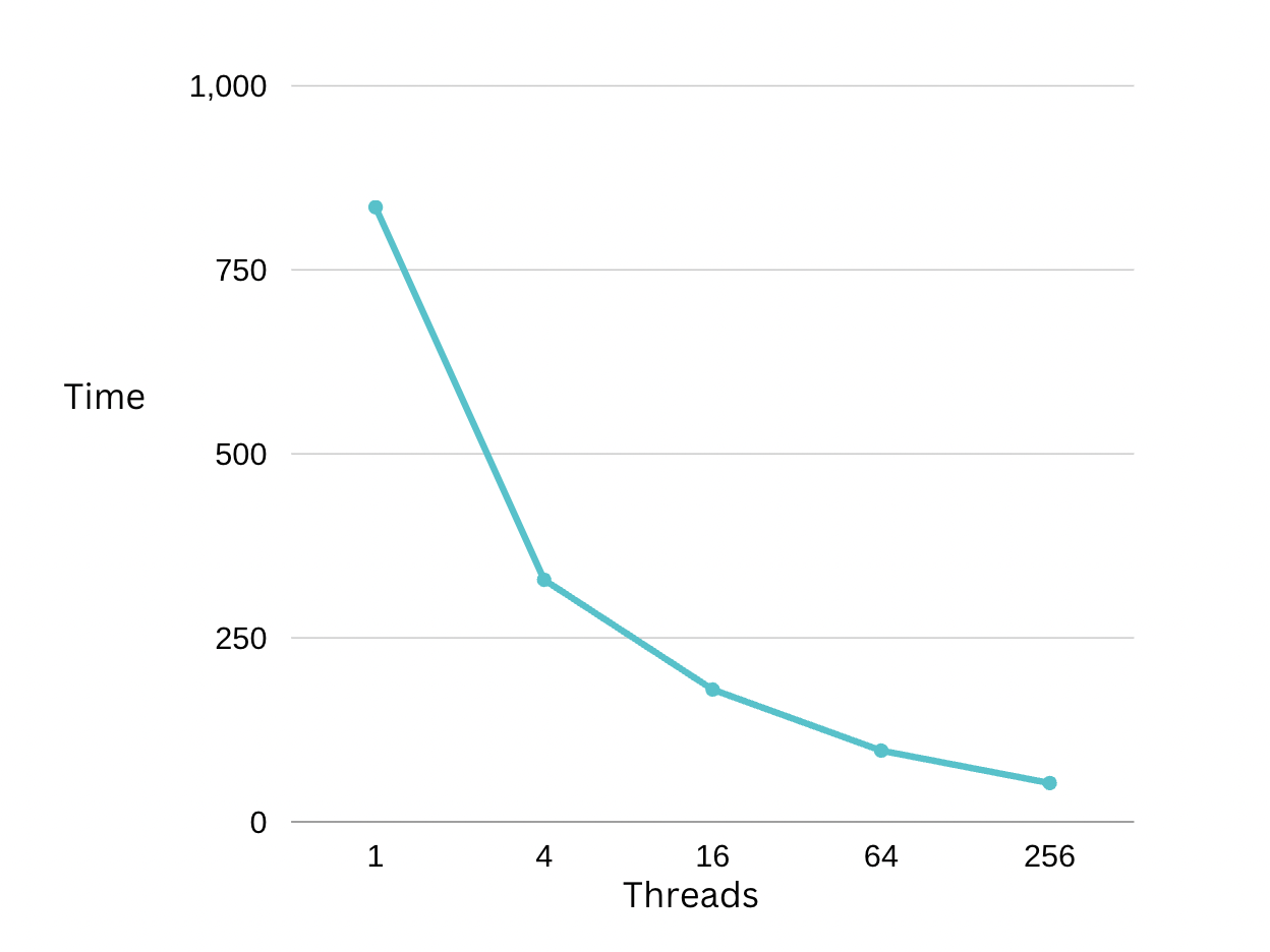
• From this plot, we see that a larger number of threads brings a better execution time. However, the margin of time shrink tends to decrease as more threads are introduced.

The Shared Output Variables Method

• $p \times p$ threads, each thread $(i,j)$ “owning” the computation of an $A(i,j)$ block, is responsible for calculating its matrix product of corresponding tile from $B$ and writing the (intermediate) results to $C(i,j)$.

Results

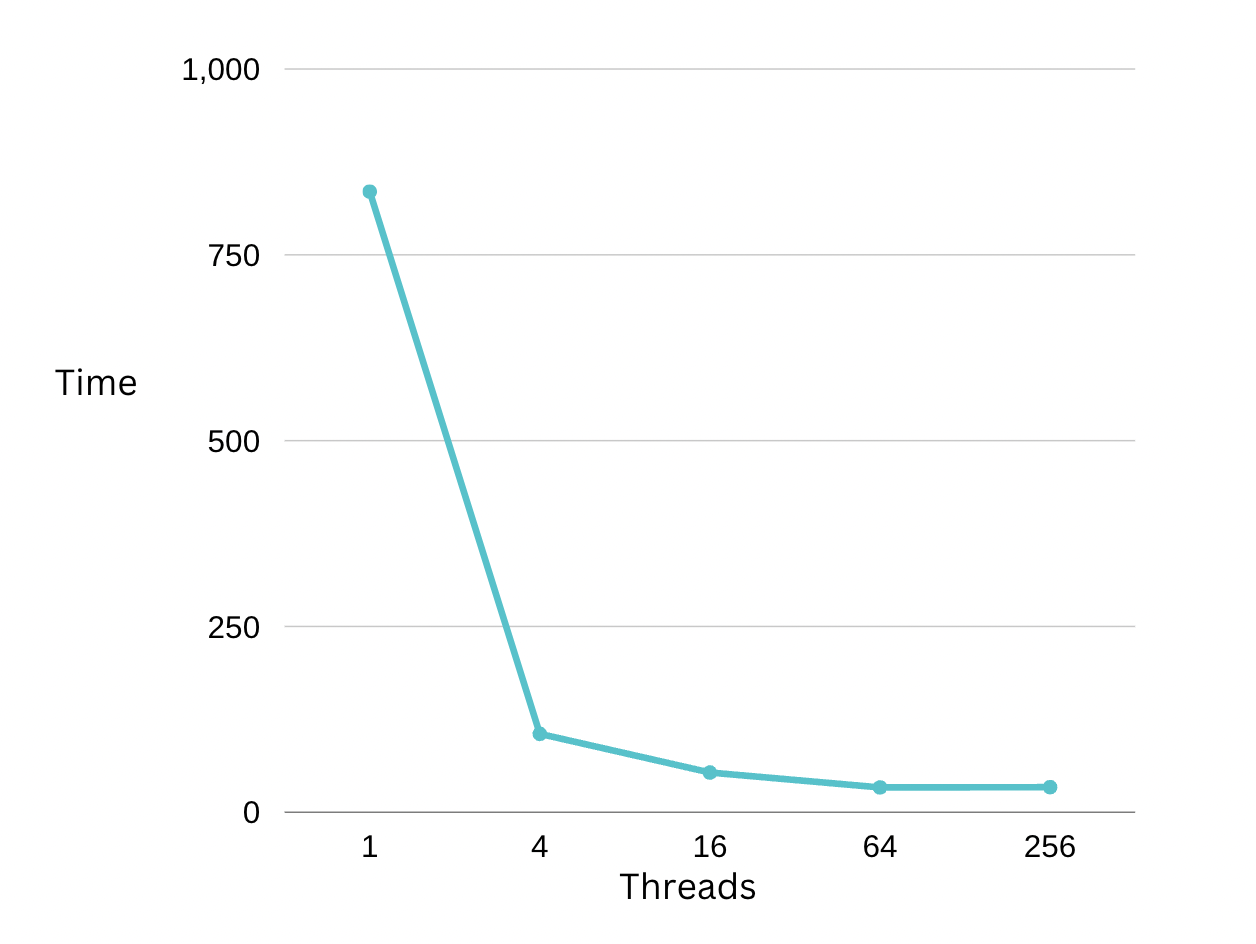
• thread = 1 (Using lab 1's result):

  Number of FLOPs = 137438953472, Execution time = 835.089545 sec,
  164.579900 MFLOPs per sec
  C[100][100]=879616000.000000
• threads = 4:

  Number of FLOPs = 137438953472, Execution time = 105.497530 sec,
  1302.769396 MFLOPs per sec
  C[100][100]=879616000.000000
• threads = 16:

  Number of FLOPs = 137438953472, Execution time = 53.448009 sec,
  2571.451323 MFLOPs per sec
  C[100][100]=879616000.000000
• threads = 64:

  Number of FLOPs = 137438953472, Execution time = 33.376083 sec,
  4117.887455 MFLOPs per sec
  C[100][100]=879616000.000000
• threads = 256:

  Number of FLOPs = 137438953472, Execution time = 33.732666 sec,
  4074.357878 MFLOPs per sec
  C[100][100]=879616000.000000

Plot

Analysis

From this plot, we see all the results perform better using the shared output variables method. For using threads 4, 16, and 64, the execution time shrinks to one-third of method one's time. For threads = 256, the time taken is very similar to (even a bit higher) that of threads = 64. This is perhaps reaching the best performance we can achieve and increasing # of threads after 64 will not enhance the speed.

Problem 2

K-means Implementation

Results

1. Run time for p = 1:

   Execution time = 0.502734 sec.

2. Run time for p = 4:

   Execution time = 0.341998 sec.

3. Run time for p = 8:

   Execution time = 0.322975 sec.

4. Output Image:

   

Analysis

Both p = 4 and p = 8 are significantly faster than p = 1, (about 1.5 times faster). The speedup factor isn't proportional to the number of threads because we are only parallelizing one step of the program, and there are other steps in the algorithm that we are not parallelizing, resulting in some overheads. Therefore, we shouldn't anticipate a linear speedup.